Tricks of the Trade
(with Professor Glesser)
Parentheses in mathematics never fails to impress me. Take, for instance, the freshman dream:

FAIL!
Not only do the parentheses matter, but in nontrivial way. Another of my favorite examples is the difference between  and
and  . Just a teeny little difference that makes all the difference in the world. You see, the first function is always greater than or equal to 0. Here are their graphs:

^2")

")
Outside of  , they aren’t even close. Of course, this suggests that if you integrate them, you expect to get wildly different answers (there are some exceptions to this: try integrating both from 0 to
  ). Ah, but there is a little problem when you try to integrate, isn’t there? You can probably handle (possibly with a great deal of effort) finding an antiderivative for , but more about that in a bit. Rather oddly, there is no elementary antiderivative for . Integrating it from 0 to
  gives an example of a Fresnel integral, but already this is beyond what most of my students want to hear in calculus. So, let’s talk about what we can actually do.
C’mon, Get to the Trick
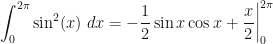
I’ve seen two reasonable ways to find the antiderivative of  : integration by parts and trig identities. The former method is actually used twice along with a little trick (I’ll get back to this later in the summer when I have a four-part series on integration by parts), while the latter requires you to remember how to convert products of sines into the cosine of a sum. I tend to use the former since I don’t have to remember anything, but the latter is probably a bit easier.
Using either method, we get  . Now, say that we want to compute
  (this is a rather common integral that seems to show up quite a bit in integral calculus and, especially, in multivariable calculus when you start doing coordinate changes). Using the fundamental theorem of calculus, we have:

and after realizing all the terms but one are 0, we see that the integral evaluates as  .
.
Some trick. I already knew how to do that.
Here is the trick. Notice that  and
and  have nearly identical graphs on
 ![[0, 2\pi]](https://s0.wp.com/latex.php?latex=%5B0%2C+2%5Cpi%5D&bg=ffffff&fg=111111&s=0&c=20201002) , the only difference is a shift. This implies that if you integrate them on , you should get the same answer, i.e.,
, the only difference is a shift. This implies that if you integrate them on , you should get the same answer, i.e., 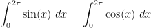 . If we square both functions, the same result holds:
  ( you better convince yourself of this before moving on).
From here, we get 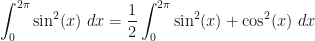 .
.
Why did we clutter up our integrand? Because, of course, we didn’t. The integrand is 1 and hence the integral evaluates to the length of the interval. In particular,  .
.
Cool, no?
But that is just one integral
True, but it is an important one. False, because obviously we can use it to compute  . Okay, that is cheating a bit. But we can actually go a little further. First, we really didn’t think hard enough about the last example. Consider the graph of
  on
on ![[0, \pi]](https://s0.wp.com/latex.php?latex=%5B0%2C+%5Cpi%5D&bg=ffffff&fg=111111&s=0&c=20201002) :
:
^2-2")
Notice that we get a full period of . Therefore, the reason what we did above worked on is that it works on and we just repeated it. Instead of the observation about  , we could also draw a rectangle with height 1 and width and remark that the area under the graph makes up precisely half the area of the rectangle, i.e.,
  . The graph makes it obvious that we could also look at only
 ![[0, \pi/2]](https://s0.wp.com/latex.php?latex=%5B0%2C+%5Cpi%2F2%5D&bg=ffffff&fg=111111&s=0&c=20201002) .
.
Before you get too excited, though, this will not work on any interval. We don’t get 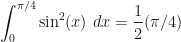 . Generally speaking, you want the interval to consist of integer multiples of
  .
.
Is that it?
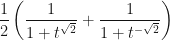
Not quite. Roger Nelsen, in a paper entitled Symmetry and Integration described the following Putnam problem:

This problem is absolutely ridiculous. Wait—did I say ridiculous? I meant ridiculously easy!!! Consider the graph of  :
:

It appears to have the same sort of symmetry as before. In fact, if we draw in few lines and do some shading, we get:

With just a modicum of thought, we see that  .
.
Whoa! What is going on here?
Actually, a lot. But let me keep it simple (there are nice generalizations of what I’ll write here); I’ll give a heuristic argument for why these things work. The key is that the functions we’ve been dealing with are symmetric about a point. Without going into too much detail, let’s just say that a function  is symmetric about a point
  , which is the midpoint of an interval
  , if for any such that
  is still in the interval , the average of
  and
and  is
is  , i.e.,
  . Truly, then, the average value of the function on is . However, we also know that the average value of any continuous function on an interval is given by
  . Therefore,
  or, equivalently,
  .
.
In our case,  ,
,  ,
,  and we get
 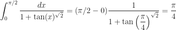 . Well, except for one thing. We still need to show the averaging property. This is just a little bit of algebra, thankfully. First, I leave it as an exercise to show that
  (try converting things into sines and cosines and using the angle addition formulas). Now, for simplicity, we write
  . The average is now given by
 , where the negative exponent comes from
  .
.
Using our fraction addition trick, this becomes 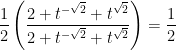 which is the required value.
^2")
")
^2-2")


