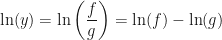
This is the second in my series on techniques I use in the classroom. Many of the things I talk about in this series are well-known, in the sense that at least 50 people know about them. What is certain is that they are not well-known to students. This entry concerns something that I want my college students to have down pat, but on which I expect them to do rather poorly: adding and subtracting fractions.
Tricks of the Trade
(with Professor Glesser)
For simplicity, let me break up addition of fractions into three categories:
- Common Denominators
- One denominator is a multiple of the other
- Other (the algebraist in me wants to write, “
 -linearly independent denominators”.)
Now, once you get by students wanting to do things like:
 (batting average addition)
then students catch on pretty quickly that the common denominator case is where they want to be. The second category of problems, exemplified here by

is only slightly more tricky. Any student who has ever needed to make change can figure out why you should think of  as
as  . In any case, I am going to assume that the students in question have mastered categories 1 and 2 (both in recognizing and computing).
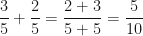
Let’s up the ante a bit and try a problem like:

I was taught to find common denominators, i.e., find a common multiple of 5 and 7 and multiply each by an appropriate factor to get two fractions with common denominators. Here for instance, we note that the least common multiple of 5 and 7 is 35. Multiplying as follows:
 and
and 
we get the new (easier) problem 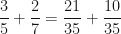 and we all know that the answer is
  . No problem, right? Well, wrong. Students routinely mess this up. First, students are usually to taught to find the least common denominator and this, for many of them, is guess-work. Second, they tend to multiply fractions incorrectly in a way they never do for category 2 problems. Third, it is just too many steps for most of them to remember and/or complete without arithmetic errors. Heck, I even messed up the above problem when I typed it up the first time.
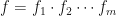
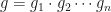
How the Pros Do It
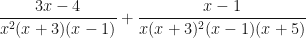
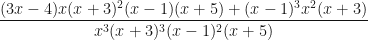
Let’s take a more general situation:  . We can always find a common denominator by multiplying the denominators¹. So, we get
  . Simply put, starting from the original problem, you cross multiply and add to get the numerator and multiply across to get the denominator.
For example, becomes easy now as the numerator is just 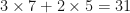 and the denominator is
  , so
, so 
Pictorially, it looks like:  Teach your students this and it will amaze you how you no longer have to interrupt the flow of a demonstration to add fractions. Show them how useful it is in the kitchen when they need to know that
  without the benefit of pencil and paper.
What about subtraction?
No problem! A similar derivation shows that to subtract, you simply cross multiply and subtract to get the numerator and multiply to get the denominator. For example, 

The biggest problem students face when doing subtraction is remembering which order you subtract (it didn’t matter for addition!) If you always start with the down-right arrow, there is no issue, though. It’s amazing. I’ve taught this to students who could hardly subtract fractions on paper, but after learning this trick, would do the problems in their head as fast as I can.
What about algebra?
It is really convenient with many algebra problems. For instance, 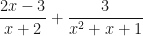 gives a lot of students fits as they can’t see how to find a common denominator. But, using this method:
 .
.
To be sure, the arithmetic is still hairy, but there is less writing than before and the student doesn’t have to think about this part, they can just do it. Now there are some cases where this method will result in some cancelling work. For example:
 .
.
A student should learn to recognize that it is much easier to multiply the first fraction by  and the second by
  and then adding. But, if they are just getting started, as long as they aren’t too overzealous about distributing, they will obtain using this method
and the cancellation is not too hard to find, leaving 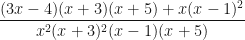 .
.
Is it really a trick?
No, not really. The formula  actually defines fraction addition. In fact, if you’re interested in a little abstract algebra, hold on to your hats.
For the advanced reader who isn’t afraid of a little jargon
There is a lovely theorem in algebra saying that every integral domain can be embedded in a field. Huh? You ate what now?
All right, let’s break it down.
AG: An integral domain is just a commutative ring where…
Poor Reader: Whoa whoa whoa. Hold on just a second, there, professor. A what?
AG: Ah, yes, a commutative ring. It is a ring that is commutative.
PR: (eyes rolling) Yes, brilliant. What the heck is a ring? (looks nervously at his or her wedding band)
AG: It is an abstract structure composed of a non-empty set and two binary operations…um, long story short, it is a set where you can add and multiply and the distributive laws hold. The only real caveat is that sometimes multiplication isn’t commutative. That means that sometimes  . Matrix multiplication is like this. In fact, the set of
  matrices forms a ring since you can add and multiply them as usual.
PR: Riiiigggghhttt (eyes are glazed over).
AG: A commutative ring is where you don’t have the multiplication problem. Then everything works just the way you want it to.
PR: Okay, let’s say for a moment I understand what you’re talking about. What is this integral domain thing then?
AG: Good question. Remember how you solve  ? You factor to get
  and then conclude that
  or
or  . How do you conclude that?
PR: Well, we know that if  then
then  or
or  .
.
AG: Precisely. Any commutative ring that has that property, we call an integral domain.
PR: That is a stupid name. I think I could do better.
AG: Yes, yes, you’re very smart; now, shut up! The theorem is that every integral domain can be embedded in a field. A field is just an integral domain where you can divide by anything other than 0 (Even in abstract algebra, except in 1 case, we are never, ever, allowed to divide by 0).
PR: What do you mean by embedded?
AG: It is a bit technical. Strictly speaking, it means that there is an injective ring homomorphism from the integral domain into a field. But just think about how every integer is also a rational number.
PR: Rational number?
AG: I’m sorry: a fraction. See if I have the integer 4, I can think of it as  and then it is a fraction. This is how we embed the integers into the rational numbers, which are a field since you can divide by fractions.
PR: You can divide by integers too. Aren’t they a field?
AG: No, because if you divide by an integer, you don’t normally get an integer. Fields have to be closed. By that, I mean that when you divide, the answer is still in the field.
PR: Hmmm. I don’t think I understand this.
AG: That’s okay. If you could really learn it in a blog post, you wouldn’t have to take an entire year of it in graduate school. The point of all this is to get at the following. To build a field from an integral domain, you take the elements of the integral domain and start writing down all fractions from those elements. You need to then explain how to add and multiply those fractions.² The answer is to define these as
and

,
which is precisely how you do it normally. Now, there is a lot more to proving the theorem. There are issues of showing this is well-defined, that the usual laws of arithmetic (e.g., associativity, commutativity, distributivity) hold and that you can produce an injective ring homomorphism. This shows though, that it is not just more computationally efficient to add this way, but that when we don’t show it, we are actually missing out on a core ingredient of a key theorem in abstract algebra.
PR: (snoring)…hmm, what, oh yes, that is a shame. Did you check your pocket for the key?
________________________________________________________________________________
¹ This will likely not give you the least common denominator, but the only cost is that you’ll have to do some cancellation at the end.
² You also need to define when two fractions are the same:  if and only if
  .
.
![y = \sqrt[3]{\dfrac{(3x-2)^2\sqrt{2x^3+1}}{x^4(x-1)}}](https://s0.wp.com/latex.php?latex=y+%3D+%5Csqrt%5B3%5D%7B%5Cdfrac%7B%283x-2%29%5E2%5Csqrt%7B2x%5E3%2B1%7D%7D%7Bx%5E4%28x-1%29%7D%7D&bg=ffffff&fg=111111&s=0&c=20201002)


 and
and  the first time and then go through it and say something like, “Well, that didn’t get us much of anywhere. What if we switch up our u and dv this time? Let’s let
  and
and  .” Then when you work it through, everything cancels out and we’re back to the original problem.
")

 . Let’s say you just happen to know the antiderivative of
  (I didn’t, although I can use integration by parts to figure it out!). You would now get:
")
")
 . Although we did integrate
  in our first post, it gave an answer of
  and we don’t want to integrate that since it we don’t know how to integrate
  (in a future post, we will resolve this last problem directly). On the other hand, if we put the
  and the natural logarithm is gone. So when does it pay to put the polynomial on the right? Whenever the derivative of the other function changes it into an
  , differentiate the
  and integrate
  .
.
 ) and which we should antidifferentiate (i.e., be our
  ). For now, I will give you that a sound choice is
 .
.

 .
. is smaller. But, I’ll grant you that life doesn’t seem much better. Essentially, we need to do integration by parts again. So, we rename things:


 .
. becomes our new
  ) and then subtract the integral of the product left to right along the bottom (
 ):
):")
")
 and antidifferentiate on the right as many times as we differentiated.
") Notice here that we are condensing quite a bit of notation with this method since we are no longer using the u, v, du, and dv notation. But, we are getting out precisely the same information. We draw diagonal left-to-right arrows to indicate which terms multiply and we superscript the arrows with alternating pluses and minuses to give the appropriate sign.
Notice here that we are condensing quite a bit of notation with this method since we are no longer using the u, v, du, and dv notation. But, we are getting out precisely the same information. We draw diagonal left-to-right arrows to indicate which terms multiply and we superscript the arrows with alternating pluses and minuses to give the appropriate sign.")
 . Following the arrows and taking account of signs, our antiderivative is
 . We simply set up the chart where, going down, we differentiate on the left and antidifferentiate on the right:
")


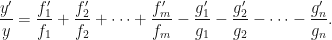
 of some common variable, say
  .
. . The typical calculus student, fooled by the simplicity of the sum rule and not having the product rule in mind, will incorrectly assert
  . Of course, differentiating shows that this answer is wrong. Why? Well, because antidifferentiation is additive but isn’t multiplicative.
 , i.e.,
  . Consequently, we could write
 .
. and
and  . This gives
 .
. .
. . Yes, it is one of those kinds of tricks. Now, I know that
  is the derivative of
  and
and  . This gives:
 .
. and
and 

 and
and 
 (or, in degrees,
  ) and their second through fourth quadrant analogues. My method is only slightly different and is likely well-known, but as most of my students have never seen it, I figure there is at least one person out there I can help. This also gives me an opportunity to throw out a useful mnemonic that naturally attaches itself to the unit circle.
 or
or 
 , starting with my palm facing in, I put down the second finger from the left and flip over my hand:

 .
.


 into any of the polynomials, you are left with 0, so it is a root. But, if that is what you do, then you won’t see the trick. When you plug 1 in, the
  as a root, but we can also immediately find the other root. How? Let’s factor. Since 1 is a root, we know that
  is a divisor of
  and so
  . Equating coefficients, we get
  and
and  . In other words, the other root is
  . Hmmm, that wasn’t so immediate; that took effort. Fine, lets start over with an arbitrary quadratic
  such that
  (implying that 1 is a root). We can factor
  and, equating coefficients, we get
  and
and  . Ah, hah! So under our assumptions, the roots are 1 and
  .
. .
.
 and
and  (that last one takes more work than the others). This isn’t quite as nice as before (not even close, actually), but if you’re into obscure formulas, this might be your cup of tea. Let me give another example of a cubic, though, that is a little more fun.
 . At this point, your
 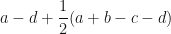 , you also get 0. Meaning that
  divides
  !
! . Checking for 0 as a root is pretty straightforward and I’ve just shown you how to find
  ? It is only slightly more complicated.
 . If this equals
  implies that
  . As before, we can factor:
  and so
  and
and  . Thus, the other root is
  . This tells us that the other root of
  .
. , you simply check whether
  .
. (rational here means an integer divided by a non-zero integer and the degree of a polynomial is the highest power of
  (where I don’t care at all about the terms in the middle) are all of the form
  where
where  divides
  and
and  divides
  . In the special case where
  , then there are only two possible rational roots:
 can be factored as
  , but
, but  are
are 
 and
and  . Just a teeny little difference that makes all the difference in the world. You see, the first function is always greater than or equal to 0. Here are their graphs:
^2")

")
 , they aren’t even close. Of course, this suggests that if you integrate them, you expect to get wildly different answers (there are some exceptions to this: try integrating both from 0 to
  ). Ah, but there is a little problem when you try to integrate, isn’t there? You can probably handle (possibly with a great deal of effort) finding an antiderivative for
 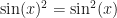 : integration by parts and trig identities. The former method is actually used twice along with a little trick (I’ll get back to this later in the summer when I have a four-part series on integration by parts), while the latter requires you to remember how to convert products of sines into the cosine of a sum. I tend to use the former since I don’t have to remember anything, but the latter is probably a bit easier.
 . Now, say that we want to compute
  (this is a rather common integral that seems to show up quite a bit in integral calculus and, especially, in multivariable calculus when you start doing coordinate changes). Using the fundamental theorem of calculus, we have:
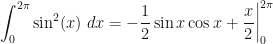

 .
. have nearly identical graphs on
 ![[0, 2\pi]](https://s0.wp.com/latex.php?latex=%5B0%2C+2%5Cpi%5D&bg=ffffff&fg=111111&s=0&c=20201002) , the only difference is a shift. This implies that if you integrate them on
, the only difference is a shift. This implies that if you integrate them on 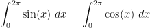 . If we square both functions, the same result holds:
  ( you better convince yourself of this before moving on).
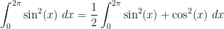 .
. .
. . Okay, that is cheating a bit. But we can actually go a little further. First, we really didn’t think hard enough about the last example. Consider the graph of
  on
on ![[0, \pi]](https://s0.wp.com/latex.php?latex=%5B0%2C+%5Cpi%5D&bg=ffffff&fg=111111&s=0&c=20201002) :
:^2-2")
 , we could also draw a rectangle with height 1 and width
  . The graph makes it obvious that we could also look at only
 ![[0, \pi/2]](https://s0.wp.com/latex.php?latex=%5B0%2C+%5Cpi%2F2%5D&bg=ffffff&fg=111111&s=0&c=20201002) .
.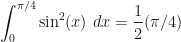 . Generally speaking, you want the interval to consist of integer multiples of
  .
.
 :
:

 .
. is symmetric about a point
  , which is the midpoint of an interval
  , if for any
  is still in the interval
  and
and  is
is  , i.e.,
  . Truly, then, the average value of the function on
  . Therefore,
  or, equivalently,
 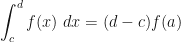 .
. ,
,  ,
,  and we get
 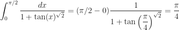 . Well, except for one thing. We still need to show the averaging property. This is just a little bit of algebra, thankfully. First, I leave it as an exercise to show that
  (try converting things into sines and cosines and using the angle addition formulas). Now, for simplicity, we write
  . The average is now given by
 , where the negative exponent comes from
  .
.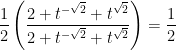 which is the required value.

